44 adding labels to excel chart
How to Use Cell Values for Excel Chart Labels - How-To Geek Select the chart, choose the "Chart Elements" option, click the "Data Labels" arrow, and then "More Options." Uncheck the "Value" box and check the "Value From Cells" box. Select cells C2:C6 to use for the data label range and then click the "OK" button. The values from these cells are now used for the chart data labels. How to Create Dynamic Chart Titles in Excel - Trump Excel Linking a Cell Value to the Chart Title. Suppose you have the data as shown below and you have created a chart using it. If you want to change the chart title, you need to manually change it by typing the text in the box. Since the chart title is static, you would have to change it again and again whenever your data is refreshed/updated.
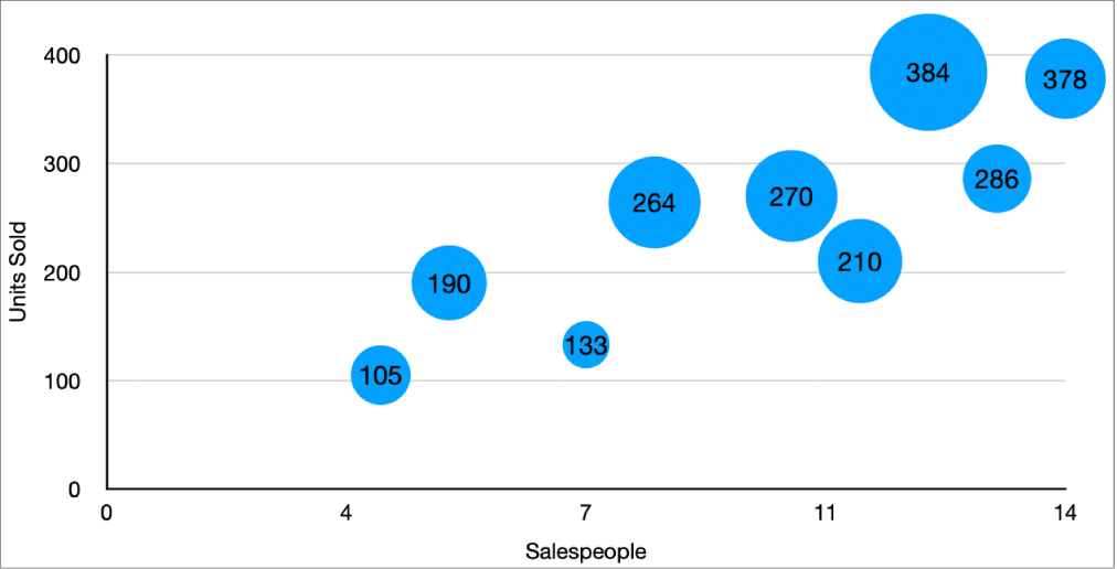
Excel: How to Create a Bubble Chart with Labels - Statology To add labels to the bubble chart, click anywhere on the chart and then click the green plus "+" sign in the top right corner. Then click the arrow next to Data Labels and then click More Options in the dropdown menu: In the panel that appears on the right side of the screen, check the box next to Value From Cells within the Label Options ...

Adding labels to excel chart
Add or remove data labels in a chart - support.microsoft.com Add data labels to a chart Click the data series or chart. To label one data point, after clicking the series, click that data point. In the upper right corner, next to the chart, click Add Chart Element > Data Labels. To change the location, click the arrow, and choose an option. How to add data labels from different column in an Excel chart? Right click the data series in the chart, and select Add Data Labels > Add Data Labels from the context menu to add data labels. 2. Click any data label to select all data labels, and then click the specified data label to select it only in the chart. 3. Add Total Value Labels to Stacked Bar Chart in Excel (Easy) Right-click on your chart and in the menu, select the Select Data menu item. In the Select Data Source dialog box, click the Add button to create a new chart series. Once you see the Edit Series range selector appear, select the data for your label series. I would also recommend naming your chart series " Total Label " so you know the ...
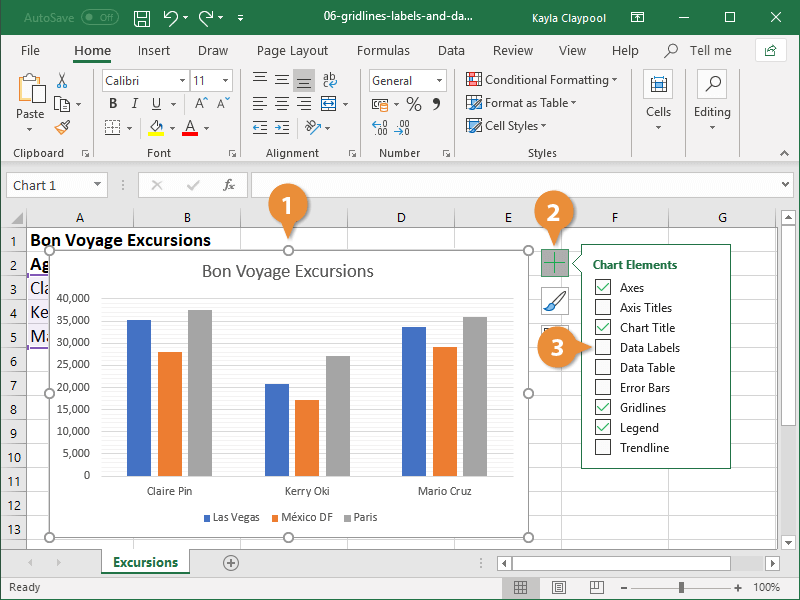
Adding labels to excel chart. How to add or move data labels in Excel chart? - ExtendOffice 1. Click the chart to show the Chart Elements button . 2. Then click the Chart Elements, and check Data Labels, then you can click the arrow to choose an option about the data labels in the sub menu. See screenshot: Waterfall Chart: Excel Template & How-to Tips | TeamGantt Adding Titles and Labels. To add a title to your chart: Click on your chart and look for “chart options” in the formatting palette. ... Gantt chart Excel template: Save time organizing your project plan with our premade Excel gantt chart template! Simply plug in your tasks and dates, and you'll have a presentation-quality Excel gantt chart. Percentage Change Chart – Excel – Automate Excel This tutorial will demonstrate how to create a Percentage Change Chart in all versions of Excel. Percentage Change – Free Template Download Download our free Percentage Template for Excel. Download Now Percentage Change Chart – Excel Starting with your Graph In this example, we’ll start with the graph that shows Revenue for the last 6… Data Labels in Excel Pivot Chart (Detailed Analysis) Add a Pivot Chart from the PivotTable Analyze tab. Then press on the Plus right next to the Chart. Next open Format Data Labels by pressing the More options in the Data Labels. Then on the side panel, click on the Value From Cells. Next, in the dialog box, Select D5:D11, and click OK.
Combining chart types, adding a second axis | Microsoft 365 Blog Jun 21, 2012 · Selecting a data set on a chart. 2. Once you have selected the Total Transactions column in the chart, click Chart Design, and then click the Change Chart button. 3. In the Change Chart Type dialog box, select the Combo, change Total Transactions to Line and click OK. Voila, you’ve created a chart with two chart types (column and line)! How to Add Labels to Scatterplot Points in Excel - Statology Step 3: Add Labels to Points Next, click anywhere on the chart until a green plus (+) sign appears in the top right corner. Then click Data Labels, then click More Options… In the Format Data Labels window that appears on the right of the screen, uncheck the box next to Y Value and check the box next to Value From Cells. Comparison Chart in Excel | Adding Multiple Series Under Graph … This window helps you modify the chart as it allows you to add the series (Y-Values) as well as Category labels (X-Axis) to configure the chart as per your need. Under Legend Entries ( S eries) inside the Select Data Source window, you need to select the … How to Add Two Data Labels in Excel Chart (with Easy Steps) Table of Contents hide. Download Practice Workbook. 4 Quick Steps to Add Two Data Labels in Excel Chart. Step 1: Create a Chart to Represent Data. Step 2: Add 1st Data Label in Excel Chart. Step 3: Apply 2nd Data Label in Excel Chart. Step 4: Format Data Labels to Show Two Data Labels. Things to Remember.
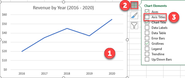
Edit titles or data labels in a chart - support.microsoft.com On a chart, click the label that you want to link to a corresponding worksheet cell. On the worksheet, click in the formula bar, and then type an equal sign (=). Select the worksheet cell that contains the data or text that you want to display in your chart. You can also type the reference to the worksheet cell in the formula bar. How to Add Text Labels in Excel Chart (4 Quick Methods) - ExcelDemy Steps: In the beginning, right-click on the data series of the chart. Next, select Add Data Labels and click Add Data Labels. Now, we can see in the screenshot below that all the data labels are added successfully to the chart. After that, right-click the data series and click Format Data Labels. Display Data Labels Above Data Markers in Excel Chart Data labels immediately appear on top of the data markers in the chart. Method 2: Use the Add Chart Element Drop-Down List. In this method, we use the Data Labels option on the Add Chart Element drop-down list, in the Chart Layout group on the Chart Design tab. Suppose we have the following Excel chart that does not have data labels. How to Add Axis Labels in Excel Charts - Step-by-Step (2022) - Spreadsheeto How to add axis titles 1. Left-click the Excel chart. 2. Click the plus button in the upper right corner of the chart. 3. Click Axis Titles to put a checkmark in the axis title checkbox. This will display axis titles. 4. Click the added axis title text box to write your axis label.
How to add or move data labels in Excel chart?
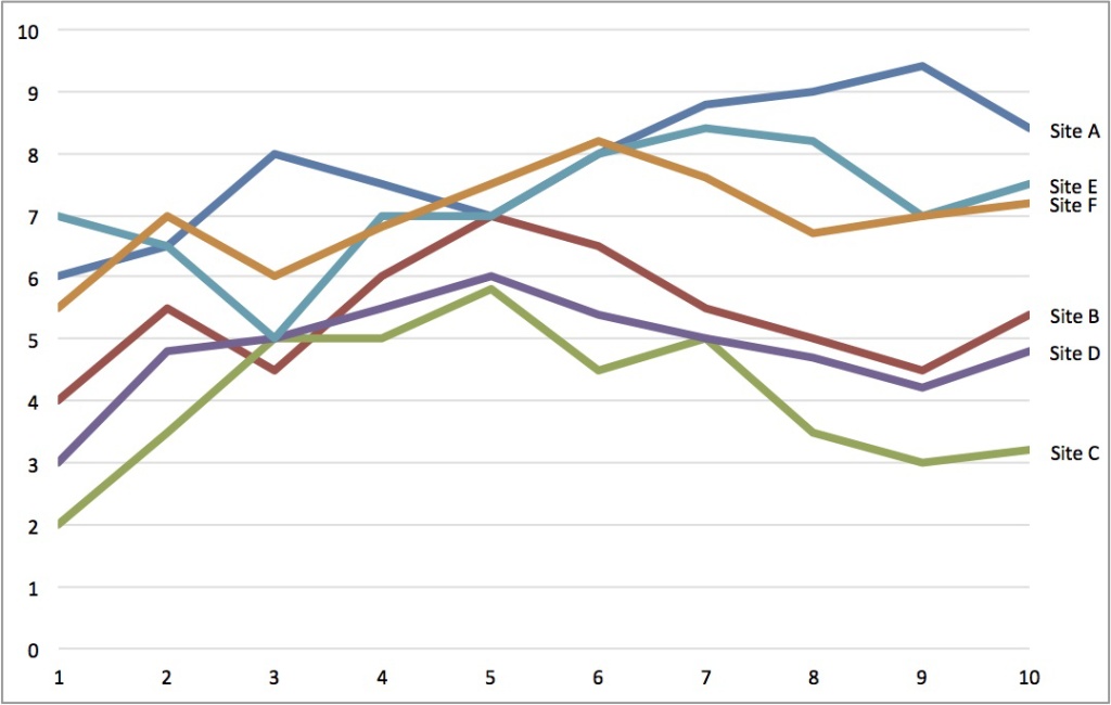
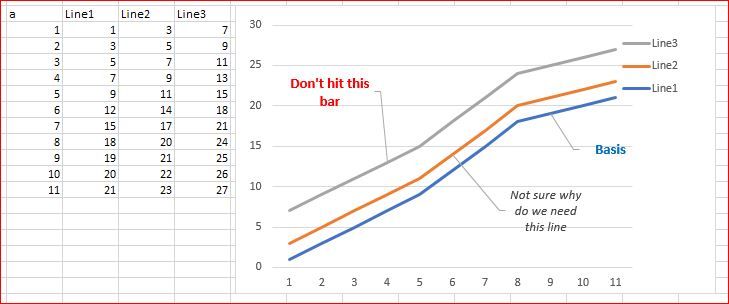
excel - Adding labels to line chart with VBA - Stack Overflow The chart that is printed looks something like this. I'm trying to figure out how to add labels to arbitrary points to the chart. Two labels to be specific. One is at the minimum value. And one is the value at any arbitrary point on x-axis. Both x-values are known and will be taken as inputs from two cells on the sheet. Something like this.

How-to Use Data Labels from a Range in an Excel Chart - Excel ...
How to Show Percentage in Excel Pie Chart (3 Ways) Sep 08, 2022 · Display Percentage in Pie Chart by Using Format Data Labels. Another way of showing percentages in a pie chart is to use the Format Data Labels option. We can open the Format Data Labels window in the following two ways. 2.1 Using Chart Elements. To active the Format Data Labels window, follow the simple steps below. Steps:

How to add live total labels to graphs and charts in Excel ...
Change axis labels in a chart in Office - support.microsoft.com In charts, axis labels are shown below the horizontal (also known as category) axis, next to the vertical (also known as value) axis, and, in a 3-D chart, next to the depth axis. The chart uses text from your source data for axis labels. To change the label, you can change the text in the source data.

How to Add Data Labels in Excel - Excelchat | Excelchat
How To Create Labels In Excel - scholarshipstudy.info Click axis titles to put a checkmark in the axis title checkbox. In this second method, we will add the x and y axis labels in excel by chart element button. Go to mailing tab > select. 47 Rows Add A Label (Form Control) Click Developer, Click Insert, And Then Click Label. 4 quick steps to add two data labels in excel chart.

Google Workspace Updates: Get more control over chart data ...
How To Add Data Labels In Excel - diemtinvn.info To do this, click the "format" tab within the "chart tools" contextual tab in the ribbon. Use the following steps to add data labels to series in a chart: Source: pakaccountants.com. Add custom data labels from the column "x axis labels". In this second method, we will add the x and y axis labels in excel by chart element button.

Dynamically Label Excel Chart Series Lines • My Online ...
How to add data labels in excel to graph or chart (Step-by-Step) Add data labels to a chart. 1. Select a data series or a graph. After picking the series, click the data point you want to label. 2. Click Add Chart Element Chart Elements button > Data Labels in the upper right corner, close to the chart. 3. Click the arrow and select an option to modify the location. 4.

Add data labels and callouts to charts in Excel 365 ...
How do you add labels to Excel? - Almanzil-Aldhakiu Manually add data labels from different column in an Excel chart. Right click the data series in the chart, and select Add Data Labels > Add Data Labels from the context menu to add data labels. Click any data label to select all data labels, and then click the specified data label to select it only in the chart. •.

Add or remove data labels in a chart
Add or remove data labels in a chart - support.microsoft.com Add data labels to a chart Click the data series or chart. To label one data point, after clicking the series, click that data point. In the upper right corner, next to the chart, click Add Chart Element > Data Labels. To change the location, click the arrow, and choose an option.

how to add data labels into Excel graphs — storytelling with data
Column Chart in Excel | How to Make a Column Chart? (Examples) Column Chart in Excel. A column chart in Excel is a chart that is used to represent data in vertical columns. The height of the column represents the value for the specific data series in a chart. The column chart represents the comparison in the form of the column from left to right. If there is a single data series, it is easy to see the ...
Directly Labeling Excel Charts - PolicyViz
Broken Y Axis in an Excel Chart - Peltier Tech Nov 18, 2011 · The primary axis then bisects the chart and the secondary is at the bottom of the chart. I usually hide the labels and often the tick marks for the primary axis. ... surely you would agree that adding some kind of indicator of the break would make the chart less misleading. ... Broken Y Axis in an Excel Chart – Peltier Tech Blog Moreover, how ...

How to Change Excel Chart Data Labels to Custom Values?
How to Add Data Labels to an Excel 2010 Chart - dummies Select where you want the data label to be placed. Data labels added to a chart with a placement of Outside End. On the Chart Tools Layout tab, click Data Labels→More Data Label Options. The Format Data Labels dialog box appears.

Excel: How to Create a Bubble Chart with Labels - Statology
About Our Coalition - Clean Air California About Our Coalition. Prop 30 is supported by a coalition including CalFire Firefighters, the American Lung Association, environmental organizations, electrical workers and businesses that want to improve California’s air quality by fighting and preventing wildfires and reducing air pollution from vehicles.

Change the format of data labels in a chart
How to Add Data Labels to Scatter Plot in Excel (2 Easy Ways) - ExcelDemy At first, go to the sheet Chart Elements. Then, select the Scatter Plot already inserted. After that, go to the Chart Design tab. Later, select Add Chart Element > Data Labels > None. This is how we can remove the data labels. Read More: Use Scatter Chart in Excel to Find Relationships between Two Data Series. 2.
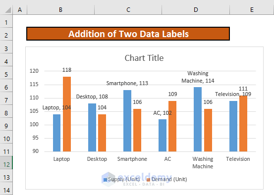
How to Add Two Data Labels in Excel Chart (with Easy Steps ...
Custom Chart Data Labels In Excel With Formulas - How To Excel At Excel Select the chart label you want to change. In the formula-bar hit = (equals), select the cell reference containing your chart label's data. In this case, the first label is in cell E2. Finally, repeat for all your chart laebls. If you are looking for a way to add custom data labels on your Excel chart, then this blog post is perfect for you.

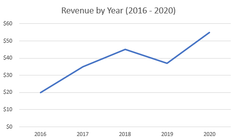
How to Add Axis Titles in a Microsoft Excel Chart
How to Add Axis Label to Chart in Excel - Sheetaki Method 1: By Using the Chart Toolbar. Select the chart that you want to add an axis label. Next, head over to the Chart tab. Click on the Axis Titles. Navigate through Primary Horizontal Axis Title > Title Below Axis. An Edit Title dialog box will appear. In this case, we will input "Month" as the horizontal axis label. Next, click OK. You ...
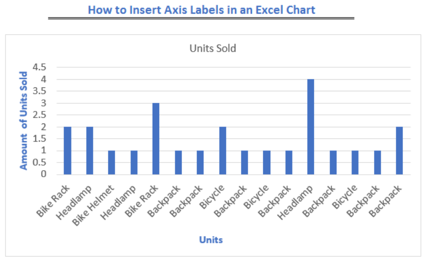
How to Insert Axis Labels In An Excel Chart | Excelchat
How to add axis label to chart in Excel? - ExtendOffice Select the chart that you want to add axis label. 2. Navigate to Chart Tools Layout tab, and then click Axis Titles, see screenshot: 3.

Adding rich data labels to charts in Excel 2013 | Microsoft ...
Add Total Value Labels to Stacked Bar Chart in Excel (Easy) Right-click on your chart and in the menu, select the Select Data menu item. In the Select Data Source dialog box, click the Add button to create a new chart series. Once you see the Edit Series range selector appear, select the data for your label series. I would also recommend naming your chart series " Total Label " so you know the ...
Add Percent Labels to a Bar Chart
How to add data labels from different column in an Excel chart? Right click the data series in the chart, and select Add Data Labels > Add Data Labels from the context menu to add data labels. 2. Click any data label to select all data labels, and then click the specified data label to select it only in the chart. 3.
How to Add Axis Labels to a Chart in Excel | CustomGuide
Add or remove data labels in a chart - support.microsoft.com Add data labels to a chart Click the data series or chart. To label one data point, after clicking the series, click that data point. In the upper right corner, next to the chart, click Add Chart Element > Data Labels. To change the location, click the arrow, and choose an option.

how to add data labels into Excel graphs — storytelling with data
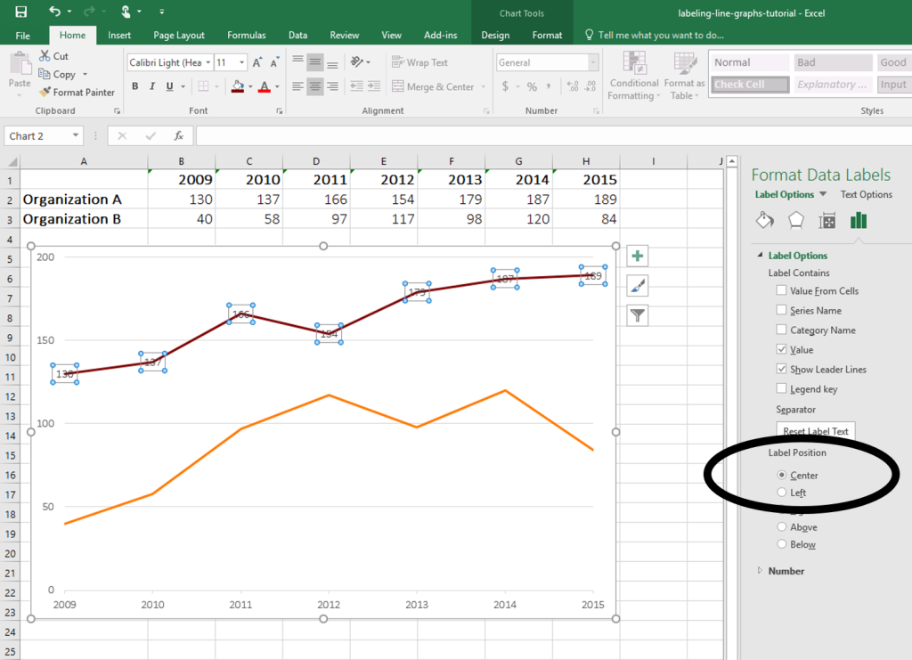
How to Place Labels Directly Through Your Line Graph in ...

How to Add Two Data Labels in Excel Chart (with Easy Steps ...

How to add data labels from different column in an Excel chart?

Excel Add Axis Label on Mac | WPS Office Academy

How to Make Pie Chart with Labels both Inside and Outside ...
How to add Axis Labels (X & Y) in Excel & Google Sheets ...
How to add Axis Labels (X & Y) in Excel & Google Sheets ...

Add Labels ON Your Bars
Change the look of chart text and labels in Numbers on Mac ...

Excel Charts: Dynamic Label positioning of line series

Microsoft Excel Tutorials: Add Data Labels to a Pie Chart
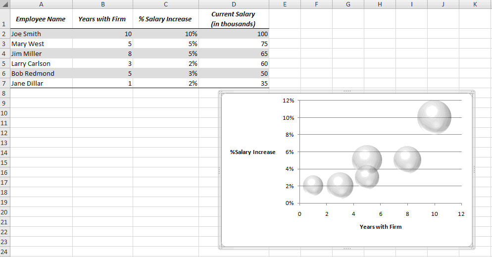
Add data labels to your Excel bubble charts | TechRepublic
Move and Align Chart Titles, Labels, Legends with the Arrow ...
Line charts: Moving the legends next to the line - Microsoft ...

Add a Data Callout Label to Charts in Excel 2013 – Software ...
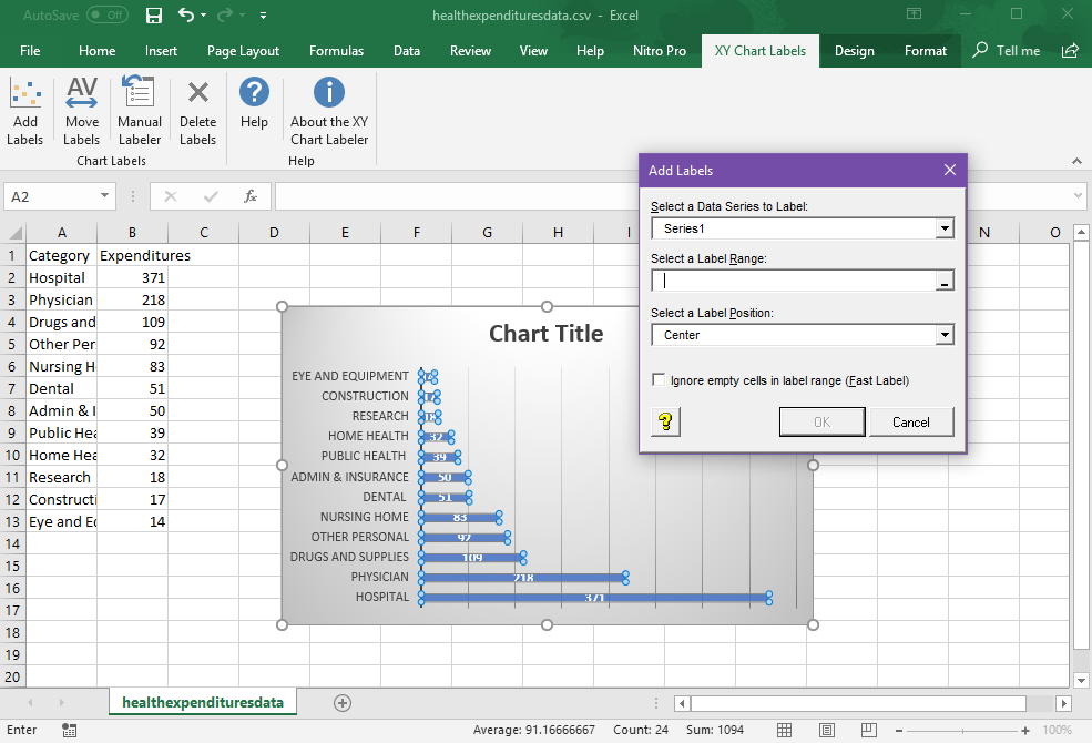
Add Labels to XY Chart Data Points in Excel with XY Chart Labeler
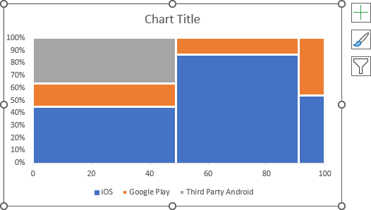
How to add labels to the Marimekko chart - Microsoft Excel 365

Adding rich data labels to charts in Excel 2013 | Microsoft ...

Add or remove data labels in a chart

microsoft excel - Adding data label only to the last value ...

Excel charts: add title, customize chart axis, legend and ...

Add label to Excel chart line • AuditExcel.co.za MS Excel ...

Adding rich data labels to charts in Excel 2013 | Microsoft ...
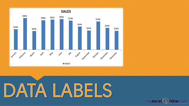
Adding Data Labels To An Excel Chart | MyExcelOnline
Post a Comment for "44 adding labels to excel chart"