41 multiple data labels excel pie chart

Pie Chart in Excel | How to Create Pie Chart - EDUCBA Pie Chart in Excel is used for showing the completion or main contribution of different segments out of 100%. It is like each value represents the portion of the Slice from the total complete Pie. For Example, we have 4 values A, B, C and D. How to fix wrapped data labels in a pie chart - Sage Intelligence Right click on the data label and select Format Data Labels. 2. Select Text Options > Text Box > and un-select Wrap text in shape. 3. The data labels resize to fit all the text on one line. 4. Alternatively, by double-clicking a data label, the handles can be used to resize the label to wrap words as desired. This can be done on all data labels ...

Edit titles or data labels in a chart - support.microsoft.com The first click selects the data labels for the whole data series, and the second click selects the individual data label. Right-click the data label, and then click Format Data Label or Format Data Labels. Click Label Options if it's not selected, and then select the Reset Label Text check box. Top of Page

Multiple data labels excel pie chart

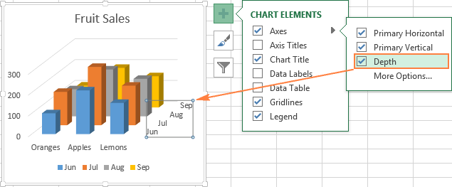
Pie Charts in Excel - How to Make with Step by Step Examples Task b: Add data labels and data callouts. Step 3: Right-click the pie chart and expand the "add data labels" option. Next, choose "add data labels" again, as shown in the following image. Step 4: The data labels are added to the chart, as shown in the following image. How to create a creative multi-layer Doughnut Chart in Excel The doughnut chart is a better version of the pie chart. While most people still use pie charts when they build reports and dashboards, the doughnut chart is the only reasonable choice for circular charts in a dashboard in my opinion. IMPORTANT: Do not use doughnut charts if you have a big amount of data points to display. A recommended amount ... Select all Data Labels at once - Microsoft Community AFAIK it has never been possible to select all data labels (if there are multiple series) You might be able to use code like this. Sub DL () Dim ocht As Chart. Dim ser As Series. Dim opt As Point. Dim s As Long. Dim p As Long. Set ocht = ActiveWindow.Selection.ShapeRange (1).Chart.

Multiple data labels excel pie chart. Create two data labels in pie chart? | MrExcel Message Board The boss wants an icon in each data label of a 6-slice pie chart. I can insert the image into the label but it often covers the text and value. Can I create a label for text/value and a second for the image? I can't put any of these values into the pie slice because some of the slices are quite small (<5%) and the data or image are not ... Create Multiple Pie Charts in Excel using Worksheet Data and VBA Here in this post I'll show you an example on how to create multiple Pie charts in Excel using your worksheet data and VBA. Click to enlarge the image! Microsoft Chart Object for Excel provides all the necessary properties and methods to create charts in your Excel workbook, efficiently. You can create charts on your worksheet or create ... How to Setup a Pie Chart with no Overlapping Labels - Telerik.com Setup a Pie Chart with no overlapping labels. In Design view click on the chart series. The Properties Window will load the selected series properties. Change the DataPointLabelAlignment property to OutsideColumn. Set the value of the DataPointLabelOffset property to a value, providing enough offset from the pie, depending on the chart size (i ... How to display leader lines in pie chart in Excel? - ExtendOffice To display leader lines in pie chart, you just need to check an option then drag the labels out. 1. Click at the chart, and right click to select Format Data Labels from context menu. 2. In the popping Format Data Labels dialog/pane, check Show Leader Lines in the Label Options section. See screenshot: 3.

How to Make a Pie Chart in Excel (Only Guide You Need) To do this select the More Options from Data labels under the Chart Elements or by selecting the chart right click on to the mouse button and select Format Data Labels. This will open up the Format Data Label option on the right side of your worksheet. Click on the percentage. If you want the value with the percentage click on both and close it. How to Combine or Group Pie Charts in Microsoft Excel Click on the first chart and then hold the Ctrl key as you click on each of the other charts to select them all. Click Format > Group > Group. All pie charts are now combined as one figure. They will move and resize as one image. Choose Different Charts to View your Data How to Create and Format a Pie Chart in Excel - Lifewire Select the plot area of the pie chart. Right-click the chart. Select Add Data Labels . Select Add Data Labels. In this example, the sales for each cookie is added to the slices of the pie chart. Change Colors When a chart is created in Excel, or whenever an existing chart is selected, two additional tabs are added to the ribbon. How to add two data labels for the same data on a pie chart? On the "Dashboard" sheet create a white circle and lay it over your circle graph. Right click it and select "Edit Text." When the cursor appears, click the formula bar and enter: =Calculation!C1. Format and align the text as desired. Next make a text box beneath the pie chart and using the same method as above set the text equal to Calculation ...

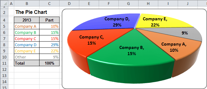
Create a multi-level category chart in Excel - ExtendOffice Create a multi-level category chart in Excel A multi-level category chart can display both the main category and subcategory labels at the same time. When you have values for items that belong to different categories and want to distinguish the values between categories visually, this chart can do you a favor. Multiple data labels (in separate locations on chart) Re: Multiple data labels (in separate locations on chart) You can do it in a single chart. Create the chart so it has 2 columns of data. At first only the 1 column of data will be displayed. Move that series to the secondary axis. You can now apply different data labels to each series. Attached Files 819208.xlsx‎ (13.8 KB, 265 views) Download Excel Pie Chart Multiple Labels | Daily Catalog Add or remove data labels in a chart. Preview. 6 hours ago On the Design tab, in the Chart Layouts group, click Add Chart Element, choose Data Labels, and then click None.Click a data label one time to select all data labels in a data series or two times to select just one data label that you want to delete, and then press DELETE. Right-click a data label, and then click Delete. Everything You Need to Know About Pie Chart in Excel Start with selecting your data in Excel. If you include data labels in your selection, Excel will automatically assign them to each column and generate the chart. Go to the INSERT tab in the Ribbon and click on the Pie Chart icon to see the pie chart types. Click on the desired chart to insert. In this example, we're going to be using Pie.

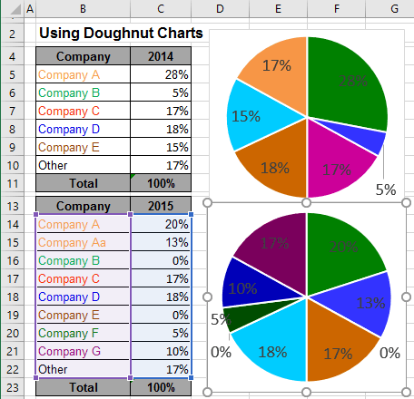
Using Pie Charts and Doughnut Charts in Excel

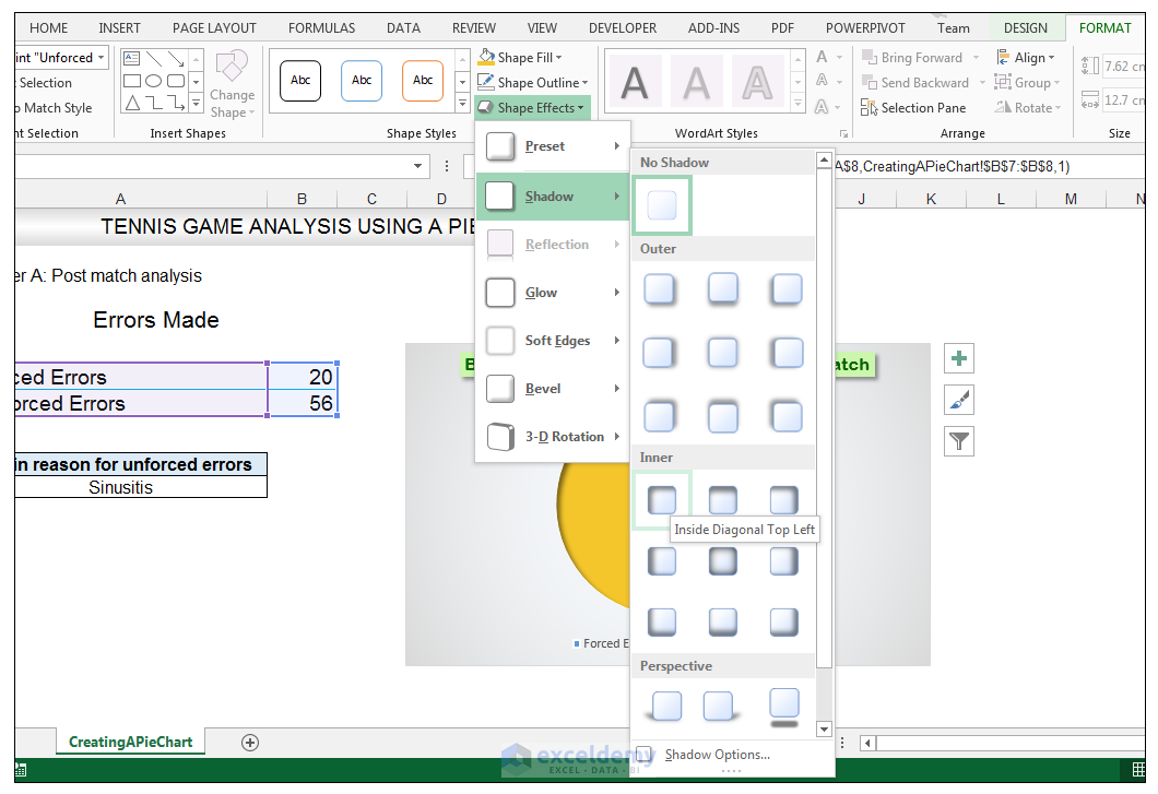
Creating Pie Chart and Adding/Formatting Data Labels (Excel) Creating Pie Chart and Adding/Formatting Data Labels (Excel)

Lesson 2 | How to Create Charts Using Microsoft Excel Tutorial

How to Create a Pie Chart in Excel - Smartsheet To create a pie chart in Excel 2016, add your data set to a worksheet and highlight it. Then click the Insert tab, and click the dropdown menu next to the image of a pie chart. Select the chart type you want to use and the chosen chart will appear on the worksheet with the data you selected.

How to Make a Pie Chart in Excel & Add Rich Data Labels to The Chart!

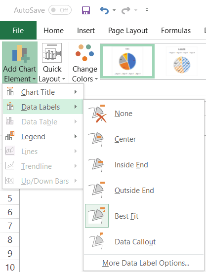
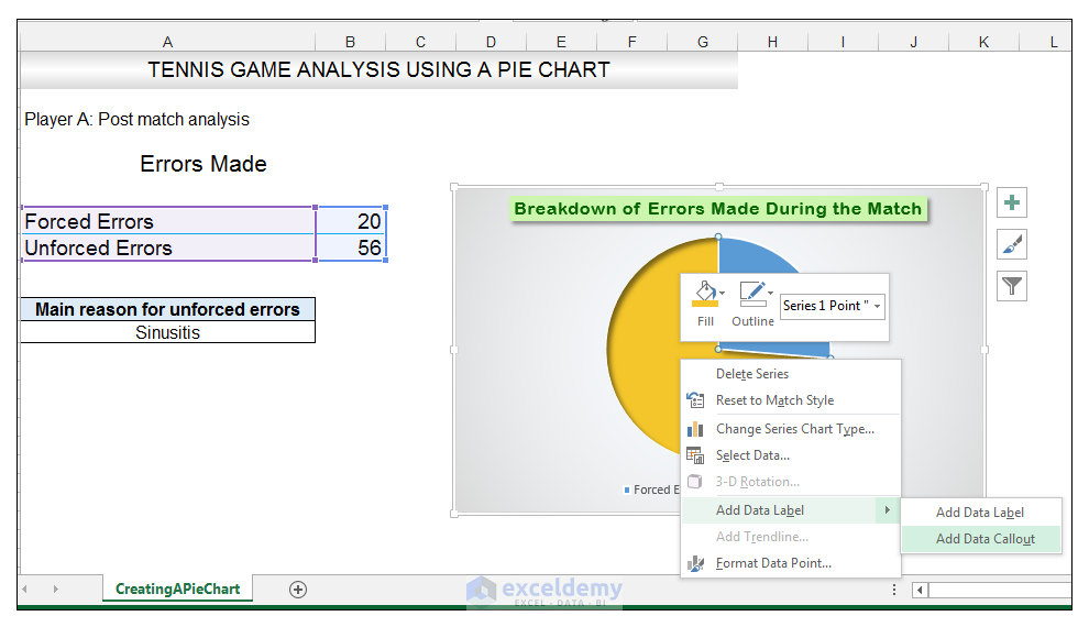
Add or remove data labels in a chart - support.microsoft.com Click the data series or chart. To label one data point, after clicking the series, click that data point. In the upper right corner, next to the chart, click Add Chart Element > Data Labels. To change the location, click the arrow, and choose an option. If you want to show your data label inside a text bubble shape, click Data Callout.

How to make a pie chart in Excel

Create a Pie Chart in Excel (In Easy Steps) - Excel Easy Create the pie chart (repeat steps 2-3). 7. Click the legend at the bottom and press Delete. 8. Select the pie chart. 9. Click the + button on the right side of the chart and click the check box next to Data Labels. 10. Click the paintbrush icon on the right side of the chart and change the color scheme of the pie chart.

Excel 3-D Pie Charts - Microsoft Excel undefined

Formatting data labels and printing pie charts on Excel for Mac 2019 ... Here's a work around I found for printing pie charts. Still can't find a solution for formatting the data labels. 1. When printing a pie chart from Excel for mac 2019, MS instructions are to select the chart only, on the worksheet > file > print. Excel is supposed to print the chart only (not the data ) and automatically fit it onto one page.

How to Make a PIE Chart in Excel (Easy Step-by-Step Guide)

Adding data labels to a pie chart - OzGrid Free Excel/VBA Help Forum Excel General. Adding data labels to a pie chart. Laplacian; Feb 24th 2005 ... Adding data labels to a pie chart. Instead of HasDataLabels try ApplyDataLabels, HasDataLabels is not a property of a chart. ... I tried recording multiple macros (create the chart from scratch, modify a created chart, etc.) and still nothing about labels. The macros ...

How to Create a Pie Chart in Microsoft Excel

Add data labels and callouts to charts in Excel 365 | EasyTweaks.com The steps that I will share in this guide apply to Excel 2021 / 2019 / 2016. Step #1: After generating the chart in Excel, right-click anywhere within the chart and select Add labels . Note that you can also select the very handy option of Adding data Callouts.

How to Make a PIE Chart in Excel (Easy Step-by-Step Guide)

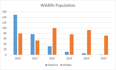
Plot Multiple Data Sets on the Same Chart in Excel Follow the below steps to implement the same: Step 1: Insert the data in the cells. After insertion, select the rows and columns by dragging the cursor. Step 2: Now click on Insert Tab from the top of the Excel window and then select Insert Line or Area Chart. From the pop-down menu select the first "2-D Line".

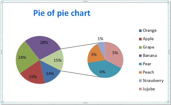
How to create pie of pie or bar of pie chart in Excel?

Solved: Show multiple data lables on a chart - Power BI For example, I'd like to include both the total and the percent on pie chart. Or instead of having a separate legend include the series name along with the % in a pie chart. I know they can be viewed as tool tips, but this is not sufficient for my needs. Many of my charts are copied to presentations and this added data is necessary for the end ...

How to make a pie chart in Excel

Select all Data Labels at once - Microsoft Community AFAIK it has never been possible to select all data labels (if there are multiple series) You might be able to use code like this. Sub DL () Dim ocht As Chart. Dim ser As Series. Dim opt As Point. Dim s As Long. Dim p As Long. Set ocht = ActiveWindow.Selection.ShapeRange (1).Chart.

Column Chart in Excel - Easy Excel Tutorial

How to create a creative multi-layer Doughnut Chart in Excel The doughnut chart is a better version of the pie chart. While most people still use pie charts when they build reports and dashboards, the doughnut chart is the only reasonable choice for circular charts in a dashboard in my opinion. IMPORTANT: Do not use doughnut charts if you have a big amount of data points to display. A recommended amount ...