39 excel chart hide zero labels
How to suppress 0 values in an Excel chart | TechRepublic You can hide the 0s by unchecking the worksheet display option called Show a zero in cells that have zero value. Here's how: Click the File tab and choose Options. In Excel 2007, click the Office... Hiding data labels with zero values | MrExcel Message Board Right click on a data label on the chart (which should select all of them in the series), select Format Data Labels, Number, Custom, then enter 0;;; in the Format Code box and click on Add. If your labels are percentages, enter 0%;;; or whatever format you want, with ;;; after it. With stacked column charts, you have to do this for each series ...
How can I hide 0-value data labels in an Excel Chart? Right click on a label and select Format Data Labels. Go to Number and select Custom. Enter #"" as the custom number format. Repeat for the other series labels. Zeros will now format as blank. NOTE This answer is based on Excel 2010, but should work in all versions Share Improve this answer edited Jun 12, 2020 at 13:48 Community Bot 1
Excel chart hide zero labels
How to hide zero data labels in chart in Excel? - ExtendOffice In the Format Data Labelsdialog, Click Numberin left pane, then selectCustom from the Categorylist box, and type #""into the Format Codetext box, and click Addbutton to add it to Typelist box. See screenshot: 3. Click Closebutton to close the dialog. Then you can see all zero data labels are hidden. Excel: Hide Zeros & Other Custom Number Formatting Tricks To show a plus sign before the positive numbers, use +0;-0;0. If you type a second semicolon and leave out the final formatting code, Excel will suppress the display of zero values. For example, 0;-0; will show positive and negative numbers but hide zeros. Note that the final semicolon is a subtle but important difference from using 0;0. I do not want to show data in chart that is "0" (zero) If your data doesn't have filters, you can switch them on by clicking Data > Sort & Filter > Filter on the Excel Ribbon. You can filter out the zero values by unchecking the box next to 0 in the filter drop-down. After you click OK all of the zero values disappear (although you can always bring them back using the same filter).
Excel chart hide zero labels. How can I hide 0-value data labels in an Excel Chart? How can I hide 0-value data labels in an Excel Chart? Right click on a label and select Format Data Labels. Go to Number and select Custom. Enter #"" as the custom number format. Repeat for the other series labels. Zeros will now format as blank. NOTE This answer is based on Excel 2010, but should work in all versions Hide data labels with low values in a chart - Excel Help Forum Hide data labels with low values in a chart. To hide chart data labels with zero value I can use the custom format 0%;;;, But is there also a possibility to hide data labels in a chart with values lower that a certain predefined number (e.g. hide all labels < 2%)? Register To Reply. 03-29-2013, 12:06 PM #2. Andy Pope. How to Quickly Remove Zero Data Labels in Excel - Medium In this article, I will walk through a quick and nifty "hack" in Excel to remove the unwanted labels in your data sets and visualizations without having to click on each one and delete manually.... How to Hide Zero Values on an Excel Chart - YouTube
Excel Pie Chart Labels on Slices: Add, Show & Modify Factors First of all, double-click on the data labels on the pie chart. As a result, a side window called Format Data Labels will appear. Then, go to the drop-down of the Label Options to Label Options tab. After that, check the Percentages option and uncheck all other options. You will get the percentages in the data labels. How can I hide segment labels for "0" values? - think-cell If the chart is complex or the values will change in the future, an Excel data link (see Excel data links) can be used to automatically hide any labels when the value is zero ("0"). Open your data source. Use cell references to read the source data and apply the Excel IF function to replace the value "0" by the text "Zero". Create a think-cell ... Hide zero value data labels for excel charts (with category name) Hide zero value data labels for excel charts (with category name) I'm trying to hide data labels for an excel chart if the value for a category is zero. I already formatted it with a custom data label format with #%;;; As you can see the data label for C4 and C5 is still visible, but I just need the category name if there is a value. Excel - charts - cannot hide the filter buttons in the chart ... Excel - charts - cannot hide the filter buttons in the chart. Hi, In Excel 2019 I was able to hide the filters buttons in the chart (right-click on the button and choose 'hide all buttons' from the menu) I needed that because I'm filtering via Slicers. Is there a way to hide them in Excel 365? right-click on the filter button won't open any menu.
Hide text labels of X-Axis in Excel - Stack Overflow Based on this data I created a bar chart looking like this: All this works fine so far. Now I want to hide the text labels of the X-Axis. Therefore I tried this: Step 1: Click on Format Axis Step 2: Click on Number Step 3: Go to Custom Step 4: Add ;;; into line Format Code. However, this only works if the labels of the X-Axis are numbers. How to hide zero in chart axis in Excel? - ExtendOffice 1. Right click at the axis you want to hide zero, and select Format Axis from the context menu. 2. In Format Axis dialog, click Number in left pane, and select Custom from Category list box, then type #"" in to Format Code text box, then click Add to add this code into Type list box. See screenshot: Add or remove data labels in a chart - support.microsoft.com On the Design tab, in the Chart Layouts group, click Add Chart Element, choose Data Labels, and then click None. Click a data label one time to select all data labels in a data series or two times to select just one data label that you want to delete, and then press DELETE. Right-click a data label, and then click Delete. How to hide points on the chart axis - Microsoft Excel 2016 This tip will show you how to hide specific points on the chart axis using a custom label format. To hide some points in the Excel 2016 chart axis, do the following: 1. Right-click in the axis and choose Format Axis... in the popup menu: 2. On the Format Axis task pane, in the Number group, select Custom category and then change the field ...
Excel Custom Chart Labels • My Online Training Hub
Hiding 0 value data labels in chart - Google Groups Try pasting this code into a code module in your workbook, go back to. the worksheet, make sure you select the chart and take. macro>vanishzerolabels>run. Sub VanishZeroLabels () For x = 1 To ActiveChart.SeriesCollection (1).Points.Count. If. ActiveChart.SeriesCollection (1).Points (x).DataLabel.Text = "0.0" Then.
34 How To Label Graphs In Excel - Labels Design Ideas 2020
Column chart: Dynamic chart ignore empty values | Exceljet To make a dynamic chart that automatically skips empty values, you can use dynamic named ranges created with formulas. When a new value is added, the chart automatically expands to include the value. If a value is deleted, the chart automatically removes the label. In the chart shown, data is plotted in one series.
35 Label The Elements In A Microsoft Excel Worksheet - Labels Design Ideas 2020
Display or hide zero values - support.microsoft.com Display or hide all zero values on a worksheet. Click the Microsoft Office Button , click Excel Options, and then click the Advanced category. Under Display options for this worksheet, select a worksheet, and then do one of the following: To display zero (0) values in cells, select the Show a zero in cells that have zero value check box.
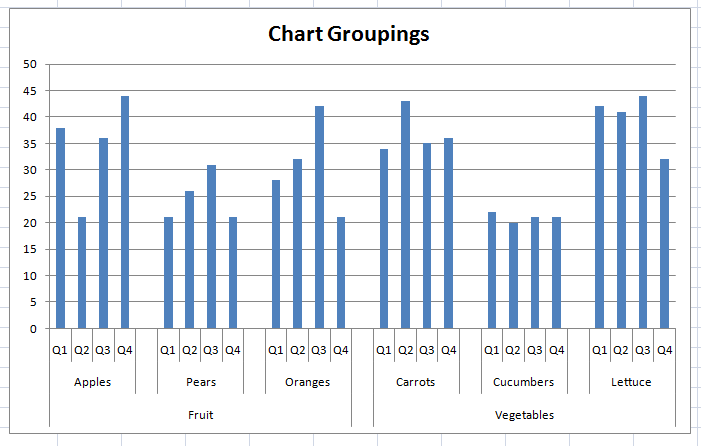
Excel Dashboard Templates Dashboard Design Examples - Excel Chart X-Axis Grouping - Excel ...
How to Hide Zero Data Labels in Excel Chart (4 Easy Ways) Now, we need to filter our dataset to hide the zero data labels in an Excel chart. First, select the range of cells B4 to C12. Then, go to the Data tab in the ribbon. After that, select Filter from the Sort & Filter group. It will filter our dataset. See the screenshot and you will see the filter drop-down option.
Post a Comment for "39 excel chart hide zero labels"