39 excel pivot table 2 row labels

Remove PivotTable Duplicate Row Labels - Excel Help Forum Re: Remove PivotTable Duplicate Row Labels. Sometimes when the cells are stored in different formats within the same column in the raw data, they get duplicated. Also, if there is space/s at the beginning or at the end of these fields, when you filter them out they look the same, however, when you plot a Pivot Table, they appear as separate ... Duplicate Items Appear in Pivot Table - Excel Pivot Tables Follow these steps to add a new field: Insert a new column in the source data, with the heading CityName. In Row 2 of the new column, enter the formula =TRIM (C2). Copy the formula down to the last row of data in the source table. If the source data is stored in an Excel Table, the formula should copy down automatically. Refresh the pivot table

How to Insert a Blank Row in Excel Pivot Table - MyExcelOnline Jan 17, 2021 · Pivot Table reports are shown in a Compact Layout format as a default and if you have two or more Items in the Row Labels (e.g.Month & Customer), then the Pivot Table report can look very clunky… There is a cool little trick that most Excel users do not know about that adds a blank row after each item, making the Pivot Table report look more ...

Excel pivot table 2 row labels

Pivot Table adding "2" to value in answer set 1) Right click your pivot table -> Pivot table options -> Data -> Change "Number of items to retain per field" to NONE 2) Wipe all rows in your data source except for the headers 3) Refresh the pivot table 4) Save, and close all instances of Excel 5) Reopen the file, and paste your data 6) Refresh the pivot table get a row label from pivot table - Microsoft Tech Community @omdl2020 . GETPIVOTDATA() doesn't work in such case, it provides data if only it is visible in PivotTable. Alternatively you may work with cube assuming you are at least on Excel 2010, as I remember it's the first which supports data model. Multiple row labels on one row in Pivot table | MrExcel Message Board I figured it out - Right click on your pivot table and choose pivot table options/display. Click on "Classic PivotTable layout" Then click on where it is subtotaling your row label and uncheck the subtotal option. D dudeshane0 New Member Joined Oct 23, 2014 Messages 1 Jan 19, 2015 #6 Gerald Higgins said:

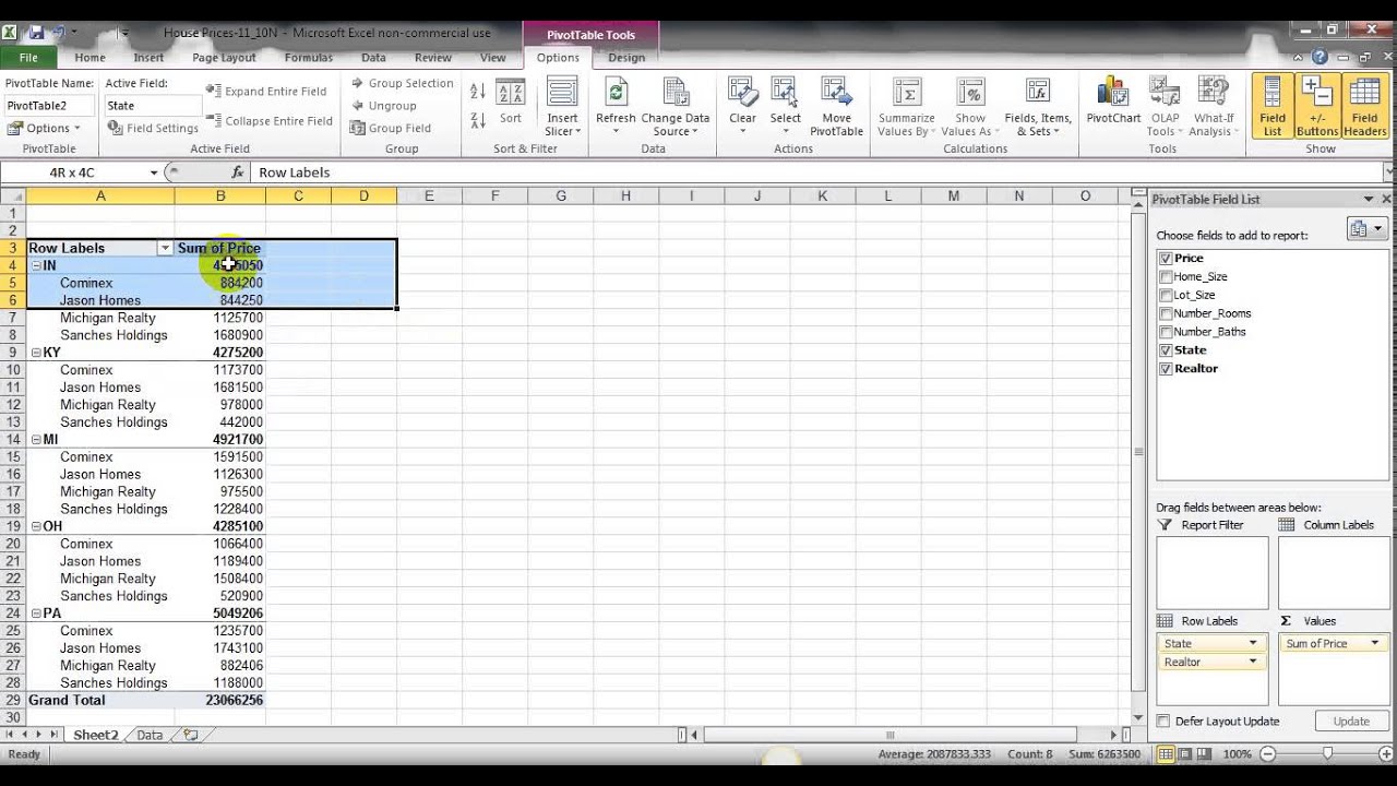
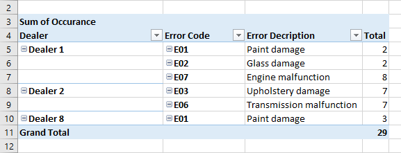
Excel pivot table 2 row labels. Pivot Table "Row Labels" Header Frustration - Microsoft Tech Community Public Sector. Internet of Things (IoT) Azure Partner Community. Expand your Azure partner-to-partner network. Microsoft Tech Talks. Bringing IT Pros together through In-Person & Virtual events. MVP Award Program. Find out more about the Microsoft MVP Award Program. Pivot Table Row Labels In the Same Line - Beat Excel! First make a pivot table with required fields. Arrange the fields as shown in left picture. Your initial table will look like right picture. Now click on "Error Code" and access field settings. First check "None" option in "Subtotals & Filters" tab to disable totals after every row. Excel Pivot Table Subtotals - Contextures Excel Tips Feb 01, 2022 · In the pivot table shown below, Service is in the Row Labels area, Lead Tech is in the Column Labels area, and Labor Cost is in the Values area. Because Service is the only field in the Row Labels area, it has no subtotal. Multiple Row Fields. When you add another field to the Row Labels area, a subtotal is automatically created for the first ... Use Excel Pivot Table as a BI tool - 云+社区 - 腾讯云 Normally, we have created a table, view in database or cube in SSAS, user can use Excel as a BI tool to display data. Here we have an Actual, Budget and Forecast data cube in SSAS. Open Excel, click "Data"->"From Other Sources"->"From Analysis Service" on Rabin menu, input SSAS server address, link to SSAS, select "PivotTable ...

Pivot table row labels side by side - Excel Tutorials - Officetuts You can copy the following table and paste it into your worksheet as Match Destination Formatting. Now, let's create a pivot table ( Insert >> Tables >> Pivot Table) and check all the values in Pivot Table Fields. Fields should look like this. Right-click inside a pivot table and choose PivotTable Options…. Check data as shown on the image below. Automatic Row And Column Pivot Table Labels - How To Excel At Excel Select the data set you want to use for your table The first thing to do is put your cursor somewhere in your data list Select the Insert Tab Hit Pivot Table icon Next select Pivot Table option Select a table or range option Select to put your Table on a New Worksheet or on the current one, for this tutorial select the first option Click Ok How to rename group or row labels in Excel PivotTable? 1. Click at the PivotTable, then click Analyze tab and go to the Active Field textbox. 2. Now in the Active Field textbox, the active field name is displayed, you can change it in the textbox. You can change other Row Labels name by clicking the relative fields in the PivotTable, then rename it in the Active Field textbox. Repeat item labels in a PivotTable - support.microsoft.com Right-click the row or column label you want to repeat, and click Field Settings. Click the Layout & Print tab, and check the Repeat item labels box. Make sure Show item labels in tabular form is selected. Notes: When you edit any of the repeated labels, the changes you make are applied to all other cells with the same label.

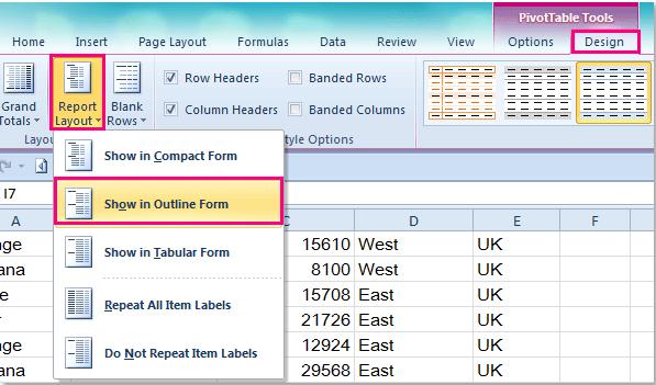
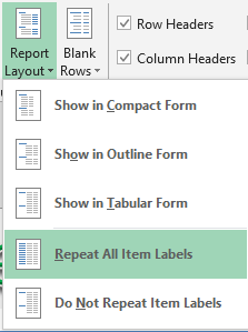
Pivot table row labels in separate columns • AuditExcel.co.za Our preference is rather that the pivot tables are shown in tabular form (all columns separated and next to each other). You can do this by changing the report format. So when you click in the Pivot Table and click on the DESIGN tab one of the options is the Report Layout. Click on this and change it to Tabular form. How to repeat row labels for group in pivot table? - ExtendOffice In Excel, when you create a pivot table, the row labels are displayed as a compact layout, all the headings are listed in one column. Sometimes, you need to convert the compact layout to outline form to make the table more clearly. But in tphe outline layout, the headings will be displayed at the top of the group. How to make row labels on same line in pivot table? Make row labels on same line with setting the layout form in pivot table As we all know, the pivot table has several layout form, the tabular form may help us to put the row labels next to each other. Please do as follows: 1. Click any cell in your pivot table, and the PivotTable Tools tab will be displayed. 2. Multi-level Pivot Table in Excel (In Easy Steps) First, insert a pivot table. Next, drag the following fields to the different areas. 1. Order ID to the Rows area. 2. Amount field to the Values area. 3. Country field and Product field to the Filters area. 4. Next, select United Kingdom from the first filter drop-down and Broccoli from the second filter drop-down.

How to repeat row labels for group in pivot table?

Pivot Table Sort by second row label - Microsoft Community Ramz Aftab Replied on May 17, 2014 Here is how you can get the results: Place your cursor on Col. B data wherever Names are. Goto Home ribbon>Editing>Sort it in either way. Alternatively, you can Sort from Pivots settings. Ramz Aftab [ MOS 77-888/82 Excel Expert ] ramzaftab [at]gmail [.]com Report abuse Was this reply helpful? Yes No

Multiple Row Filters in Pivot Tables - YouTube

Excel Pivot Table Group: Step-By-Step Tutorial To Group Or ... In fact, as mentioned in Excel 2016 Pivot Table Data Crunching: Each time you create a new pivot table in Excel 2016, Excel automatically shares the pivot cache. Pivot Cache sharing has several benefits. Most notably, as I mention above, it reduces memory requirements and file size vs. the scenario where the Pivot Cache isn't shared.

Pivot table row labels in separate columns • AuditExcel.co.za

Sum of two column labels in pivot table - Excel Help Forum Re: Sum of two column labels in pivot table. Use Slicer. (usuall Ctrl+click or Shift+click combination for multiple items) Attached Files. PT.xlsx‎ (17.1 KB, 6 views) Download.

Pivot table row labels side by side

Mail Merge Multiple Rows Into One Document :: blogshoe54 Start the Mail Merge Wizard. For this, go to the Mailings tab, and click Start Mail Merge > Step-by-Step Mail Merge Wizard. The Mail Merge panel will open on the right side of your document. In step 1, you choose the document type, which is E-mail messages, and then click Next to continue.

Repeat All Item Labels In An Excel Pivot Table | MyExcelOnline

How to Concatenate Values of Pivot Table - Basic Excel Tutorial Click insert Pivot table, on the open window select the fields you want for your Pivot table. Once you select the desired fields, go to Analyze Menu. Under calculations, choose fields, Items & Sets tab then click on calculated fields. Enter the values and click ok. Your PivotTable will display the total of combined units and price.

Pivot Tables in Excel: Beginner’s Guide

How to Create a Pivot Table in Excel: A Step-by-Step Tutorial Dec 31, 2021 · After you've completed Step 3, Excel will create a blank pivot table for you. Your next step is to drag and drop a field — labeled according to the names of the columns in your spreadsheet — into the Row Labels area. This will determine what unique identifier — blog post title, product name, and so on — the pivot table will organize ...

How to count unique values in pivot table?

How to Format Excel Pivot Table - Contextures Excel Tips May 23, 2022 · Keep Formatting in Excel Pivot Table. A pivot table is automatically formatted with a default style when you create it, and you can select a different style later, or add your own formatting. For example, in the pivot table shown below, colour has been added to the subtotal rows, and column B is narrow.

Naming Columns | CLEARIFY

Pivot table - Wikipedia Row labels are used to apply a filter to one or more rows that have to be shown in the pivot table. For instance, if the "Salesperson" field is dragged on this area then the other output table constructed will have values from the column "Salesperson", i.e. , one will have a number of rows equal to the number of "Sales Person".

Share :